Filters

DESENSITISATION · FILTER TYPES · PLACEMENT · WHEN IT IS WORTHWHILE

A node standing next to a transmitter mast can be perfectly healthy and still hear almost nothing. The chip is fine, the antenna is properly tuned, the firmware is correct — and the receiver is deaf, because there is so much power on its input that it can no longer process its own band cleanly. This chapter describes how that happens, which filters exist, what they do and do not fix, and how to work out in advance whether a filter will be a gain or a loss in your particular case.

[!NOTE] Source. Almost nothing on this page comes from the MeshCore firmware. From the firmware come only the radio parameters and the lower bound of the measured noise floor: MeshCore v1.16.0, commit 03b6ef4, 28 July 2026, file src/helpers/radiolib/RadioLibWrappers.cpp. The mast data comes from the public Dutch Antenneregister. Everything else is general radio engineering, and the level estimates are calculations with explicit assumptions — not measurements. Every figure can be recomputed with tools/filter-planning.py.

Why a receiver goes deaf

The sensitivity of a LoRa receiver is the noise floor plus the SNR that the chosen spreading factor requires. See Link Budget for that sum. What appears there as a fixed number is not fixed in practice: the noise floor is not a property of the chip but of the chip in that place.

Put the same node next to a mobile operator's site and the floor rises. Not because anything transmits on 869 MHz, but because the amplifier and mixer in the receive chain have to handle all the power the antenna collects — across the whole spectrum, not just the 62.5 kHz you care about. That rise is called desensitisation.

How much power that is can be estimated. A site in Zwolle with antennas at 30.4 m carries, according to the Antenneregister, eight bands from 773 to 3700 MHz, with powers up to 48.2 dBW. At a slant distance of 40 m and 25 dB of suppression below the main beam, that works out as:

Band	MHz	dBW	At the input
5G n28	773	34.0	−23.3 dBm
4G B20	816	34.5	−23.2 dBm
2G/4G 900	940	34.9	−24.1 dBm
L-band SDL	1474.5	36.4	−26.5 dBm
4G B3	1815	39.2	−25.5 dBm
5G n1	2160	40.5	−25.7 dBm
4G/5G 2600	2660	35.9	−32.1 dBm
5G n78	3700	48.2	−22.7 dBm
composite			−15.6 dBm

That is one sector; three sectors together sit a few dB higher. The distance and the pattern suppression are assumptions, not measurements — change the suppression to 15 or 35 dB and the whole table shifts by 10 dB. What the table does show is the order of magnitude: several tens of dB above the level at which a receiver input without preselection still behaves linearly.

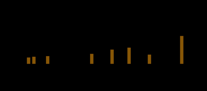
Bar height is proportional to the registered power. No carrier sits close to 869.618 MHz — the nearest is 54 MHz away. The problem is not proximity but total power.

Four ways it goes wrong

Blocking. The gain of the receive chain adjusts to the total power on the input, not to what sits in your channel. Strong signals far outside your band push the gain down and lift the effective noise floor. This is the most common cause and the only one a filter always helps against. ETSI has a requirement for it: EN 300 220-1 describes blocking and divides receivers into categories, with category 1 the most demanding and category 3 the least.

Second-order intermodulation. As soon as the input stops behaving linearly, strong signals start mixing. The difference between two transmitters can land exactly in your band. For this site:

Pair	Block width ±10 MHz	Nominal band downlink
1815 − 940	855–895 MHz — hit	845–955 MHz — hit
2660 − 1815	825–865 MHz — miss	740–885 MHz — hit

The difference between the 1800 and 900 bands lands on 869.618 MHz under any reasonable assumption. The difference between 2600 and 1800 depends on the actual channel widths: for 4G and 5G the register gives only a centre frequency, no bandwidth. Take the blocks narrow and you just miss; take the nominal bands and you hit. That product is therefore a candidate, not a certainty.

[!NOTE] The standard deliberately leaves this open. EN 300 220-2 sets no requirement for intermodulation, in order to keep testing simple; the reasoning is that the blocking requirement already covers the ability to handle strong out-of-band signals. The standard itself adds that manufacturers should assess the intermodulation risk when equipment is sited next to high-power transmitters. Exactly the situation this chapter describes.

Transmitter noise. Every transmitter produces broadband noise outside its own channel. Base stations are well filtered for this, so it is the least likely of the four — but with hundreds of kilowatts of radiated power in total, the contribution is not necessarily zero.

Passive intermodulation. Strong fields falling on corroding metal-to-metal junctions — bolts, fencing, downpipes, mounting brackets — produce mixing products there that are then re-radiated. The literature calls this the rusty bolt effect, and it is a recognised cause of receiver desensitisation at mast sites. This is the awkward variant: the product arises outside your node and is already on 869 MHz before any filter can act on it.

What a filter is

A filter passes one band and attenuates the rest. Four numbers describe it completely.

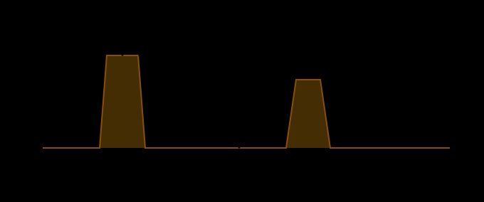
Schematic. The insertion loss is drawn exaggerated to make it visible; in reality it is a few dB against tens of dB of rejection.

Passband — where the signal is allowed through. For MeshCore in Europe that is the SRD band, 863–870 MHz. Designing it narrower gives sharper skirts but makes you sensitive to tuning and temperature.

Insertion loss — what you lose inside the passband. This causes a direct loss of sensitivity and transmit power, so it counts twice.

Rejection — what falls away outside the band. The number alone means nothing; you need to know over which frequency range it applies. A filter that achieves 40 dB up to 2 GHz and is open above that is unusable next to a 3700 MHz transmitter.

Power rating — how much transmit power the filter tolerates. The SX1262 delivers up to 22 dBm; a filter specified to +20 dBm forces you to limit the transmit power.

The resonator

Four of the five types in the next section are built from the same component. Once you know it, you can see at once why they differ so widely in Q, insertion loss and volume — and why they all share the same pitfall.

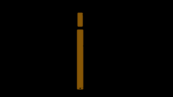
The inner conductor connects to the wall at the base and ends free at the top. The coupling loops take the signal in and out.

A quarter-wave resonator is a length of conductor inside a closed metal can, shorted to the wall at one end and free at the other. At the frequency where that conductor is exactly a quarter wavelength long, the short at the base transforms into an open end at the top: voltage at its maximum there, current at zero. That is resonance, and unlike a coil with a capacitor it is fixed by the mechanical dimensions — not by components with a tolerance and a temperature coefficient.

How long

A quarter wavelength at 869.618 MHz is 86.2 mm. In practice the conductor is made shorter and the difference is made up with capacitance above the free end: the tuning screw, or a disc. That has three consequences. The filter becomes more compact, it can be tuned without cutting metal, and the next resonance moves up. That last one is not a detail — it is exactly the control that moves the spurious passband discussed further on out of the way.

Where the Q comes from

The losses sit almost entirely in the resistance of the metal surface the current runs along. For the same stored field, more surface means less loss, which is why Q grows with the dimensions. A conductor of a centimetre and a half inside a can of eight reaches a multiple of the same resonator rolled up inside a can of two. The ranking in the table below is therefore not coincidence but geometry: from small and blunt to large and sharp.

From resonator to filter

One resonator is not yet a filter. The signal goes in and out through a loop, a tap on the conductor or a short cable. The tighter that coupling, the wider the passband and the less steep the skirts. More resonators in series make the skirts steeper and add insertion loss per resonator.

Where those resonators sit, and how they are shorted, decides the name. Rolled up inside a can it is called helical. As rods side by side in one box, shorted at alternate ends, it is interdigital; all shorted at the same end with capacitance at the top, it is combline. Each resonator in its own can, coupled with loops or short cables: a cavity filter.

The filter types

Type	Q per resonator	Insertion loss	Power	Volume
LC / ceramic	50–150	1.5–3 dB	watts	very small
SAW	multi-pole, see text	1.5–3 dB	often +10 to +20 dBm	very small
Helical	200–600	1–2 dB	watts	a small can
Interdigital / combline	800–2000	0.5–1.5 dB	tens of watts	a box
Cavity filter	2000–5000	0.3–1 dB	hundreds of watts	large and heavy

The figures are indicative and convey the order of magnitude and the relative ranking; actual values belong in the datasheet of a specific part.

LC and ceramic. Inductors and capacitors, or a ceramic block with the same effect. Cheap, small, ample power handling. The skirts are weak: at 70 MHz offset you often get no more than 15 to 25 dB. Enough against the bands above 1.5 GHz, mediocre against the 900 band.

SAW. An acoustic wave across a piezo substrate. The steepness comes not from high Q per resonator but from many poles at once, so the Q column does not apply. The steepest skirts in the smallest package, and therefore the best choice against the 900 band. Two things to watch: power handling is often limited to around +10 to +20 dBm, and attenuation far above the passband is not always specified. Check the response beyond the highest band in your surroundings.

Helical. A coil in a shielded can — effectively a rolled-up quarter-wave resonator. Considerably higher Q than LC, ample power handling, easy to build and to tune with a NanoVNA. The practical middle ground.

Interdigital and combline. Several quarter-wave rods in one rectangular box. In an interdigital filter alternate rods are shorted at opposite ends; in a combline all rods are shorted at the same end and capacitively top-loaded. High Q, low insertion loss, and the most satisfying home-built form at 868 MHz.

Cavity filter. One quarter-wave resonator per metal can, coupled with loops or short cables. The highest Q and the lowest loss, and therefore the standard in repeater duplexers where 40 dB of rejection at 600 kHz offset is required. For a node next to a mast this is overkill: your nearest interferer sits 54 MHz away, not 600 kHz. That demands volume and weight for a property you do not use.

Pass or reject

A band-pass filter passes your own band and attenuates everything else. This is nearly always the right choice, because it works against all interferers at once — including ones you have not yet identified.

A band-stop filter, or notch, does the opposite: it attenuates one narrow band and leaves the rest alone. That only makes sense when there is exactly one dominant interferer, close to your own frequency, and you know which one it is. Next to a multiband mast that is almost never the case.

A low-pass filter can be a useful supplement: cascaded behind a resonator filter it cuts everything above roughly 1 GHz, including the spurious passband discussed next.

Two pitfalls

The spurious passband. A quarter-wave resonator resonates not only at its design frequency but also at three, five and seven times that frequency. For 869.618 MHz that is 2608.9 MHz — and at this site a 2600 MHz transmitter stands 51 MHz away from it. A pure quarter-wave design would therefore pass much of that band and undermine part of its own purpose. Capacitive top loading, as in a combline, pushes that second resonance higher; a cascaded low-pass filter also solves it. A SAW filter does not show this behaviour, but has its own weak spots high in the spectrum. There is no type without a caveat — there is only the caveat you have checked.

Temperature drift. An aluminium resonator expands by roughly 23 ppm per kelvin. From −10 to +50 °C that is sixty kelvin, so about 1400 ppm, meaning a shift on the order of 1.2 MHz at 869 MHz. Do not design an outdoor filter narrower than the full SRD band of roughly 7 MHz. Then the drift is irrelevant and the tuning is far more forgiving.

Where the filter goes

The filter belongs as close to the antenna as possible, ahead of the first active component. From there, two routes.

In the shared path the transmit power passes through the filter too. With an extra switch the transmit path stays unfiltered and at full power.

In the shared path. The simplest arrangement: one filter between antenna and node. Transmit and receive both pass through it. The insertion loss counts twice, and you have to keep the transmit power under the filter's power rating.

In the receive path only. The SX1262 drives its transmit-receive switch via DIO2 — see Antenna. With an extra external switch you split the paths and place the filter in the RX branch only. The transmit path keeps full power and sees only the switch loss. The downside is an extra component, a control line, and having to work on the board.

When a filter is worthwhile

A filter does not improve everything at once. It makes the receive side better and the transmit side worse, and whether that wins on balance depends on how much desense you actually have. With 2 dB of insertion loss and a filter that forces a limit of 20 dBm, the sum becomes:

• transmit loss: 2 dB of limiting plus 2 dB of insertion loss is 4 dB, always
• receive gain: the desense minus 2 dB of insertion loss

Desense	Receive gain	Transmit loss	Net
4 dB	2 dB	4 dB	loss
6 dB	4 dB	4 dB	break-even
10 dB	8 dB	4 dB	gain
20 dB	18 dB	4 dB	gain
27 dB	25 dB	4 dB	gain

Below roughly 6 dB of desense a filter makes your situation worse. Above it the filter wins, and from about ten dB upward the outcome is no longer in doubt.

There is one asymmetry the table does not show, and it works in the filter's favour. A link is only as good as its worst direction. If only your node sits in the strong field, your reception is the binding direction and the transmit side is not. Gaining on the binding direction then outweighs losing the same amount on the other.

Measuring

Without a baseline you cannot tell afterwards what an intervention achieved.

Read the noise floor before changing anything. Thermal noise over 62.5 kHz is −126.0 dBm; with the noise figure of the receive chain added you expect a floor around −120 dBm. See Link Budget.

Compare against a second node in a quiet location, preferably with identical hardware. That is the only real reference you have.

Swap the nodes if the difference is large. If the high floor follows the location, it is the environment. If it follows the enclosure, it is the hardware and a filter gives you nothing.

Connect a dummy load instead of the antenna. If the floor drops sharply, the energy arrives through the antenna. If it stays high, it is coupling in through the enclosure, the power lead or the USB cable.

Log for a day. Blocking by the always-present carriers of a base station is essentially flat. Intermodulation moves with mobile traffic and swings between night and evening peak. That distinction determines whether a filter will help.

[!WARNING] The firmware clamps at −120 dBm. MeshCore averages 64 samples and clamps the result to a lower bound of −120 dBm; it does not report lower, even when the environment is quieter. See The LoRa Transceiver. For a node with a floor of −90 dBm the maximum demonstrable improvement is therefore 30 dB. Anyone already around −118 cannot demonstrate an improvement with this measurement — and does not need one.

A worked case

Two repeaters in Zwolle, same firmware and same settings. One stands directly below the site tabulated above, with a 6 dBi collinear, and reports a noise floor of −90 dBm. The other stands 30 metres lower, with a 3 dBi antenna, and reports −117 dBm.

Difference: 27 dB. At most 3 dB of that is attributable to the difference in antenna gain, and then only for interferers inside the 868 band; outside that band the gain figure of an 868 antenna means nothing. The rest is environment.

What that means for the high node: everything arriving weaker than roughly 27 dB above its normal threshold is lost. Translated into distance, with a propagation exponent between 2 and 3.5, it hears at roughly a sixth to a twentieth of the range it should achieve.

There is a second clue in the same installation that is easily overlooked: the BLE connection to the high node only works with the phone held almost against it. That is a different radio, a different band and a different antenna path, with the same symptom. Two independent receivers with the same complaint point at the environment, not at a defect. An 868 filter does not fix that second symptom — see below.

What a filter does not fix

Signals inside your own band. Passive intermodulation arising at 869 MHz is already inside the passband before the filter can act. If the floor stays high after installation and keeps following the traffic pattern, this is the cause, and only geometry helps: further away, lower, or an installation that is not on the same steel structure.

Other bands. An 868 filter sits in the LoRa path. BLE and WiFi have their own antenna, usually on the board, and gain nothing from it. See BLE Architecture.

Coupling outside the antenna path. Fields entering via the power lead, the USB cable or the enclosure bypass the filter entirely. Ferrites and a common-mode choke belong to the same intervention.

A poor location. A filter gives you twenty or thirty dB at best. Going thirty metres lower gave twenty-seven dB in the case above, without insertion loss and without limiting the transmit power. Filtering is the answer when you cannot move; it is not a substitute for thinking about where the node goes.

Sources

Firmware, commit 03b6ef4 (v1.16.0, 28 July 2026):

• src/helpers/radiolib/RadioLibWrappers.cpp — the measured noise floor, 64 samples, and the lower bound of −120 dBm
• platformio.ini — LORA_FREQ, LORA_BW and the maximum transmit power

In this repository:

• tools/filter-planning.py — recomputes every figure on this page and shows how sensitive it is to the assumptions

Outside the firmware:

1. ETSI EN 300 220-1 V3.1.1 — receiver categories and the description of blocking
2. ETSI EN 300 220-2 V3.1.1 — blocking limits, and the explanation of why intermodulation is deliberately not specified
3. Analog Devices — Passive Intermodulation Effects in Base Stations — the rusty bolt effect and receiver desensitisation caused by PIM
4. Antenneregister — the powers, heights and bearings of the site
5. ETSI TR 102 649-2 — subband overview for 868–870 MHz
6. Semtech SX1262 — the transmit power of the chip

Not from any source: the slant distance of 40 m, the pattern suppression of 25 dB, the block widths around the registered centre frequencies, and the indicative Q values and insertion losses per filter type. All four are marked as such in the text and in the script.

Related chapters:

• Antenna — the RF switch and the connector the filter goes between
• Link Budget — where the noise floor lands in the sum
• The LoRa Transceiver — how the firmware measures and clamps its noise floor
• Higher and stronger isn't always better — why the installation weighs more than the component
• Regulations & Duty Cycle — what you may radiate after the insertion loss is deducted

Translated from Dutch by Anthropic Claude